Peak Fit

Fit data to a composite peak model.

Inputs

• Data: Input data set

Outputs

• Fit Parameters: Best fit values for the model parameters
• Fits: Total evaluated best fit
• Residuals: Difference between Fits and Data
• Data: Input data set annotated with Fit Parameters

The Peak Fit widget computes the least-squares minimization curve fit for arbitrary, user-defined composite peak models. It outputs the best fit parameters for the defined model and the resulting total fit.

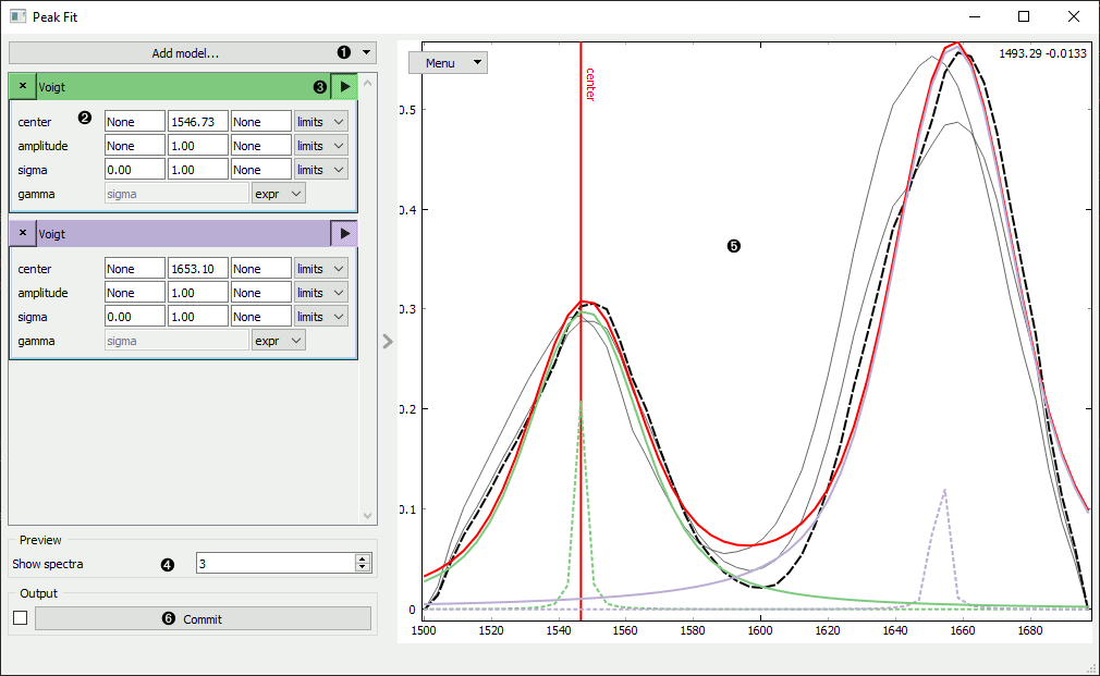
1. Add a model component from the dropdown menu.
2. Input model initial parameters and constraints.
3. Visualize the initial peak and peak color.
4. Select subsample of data for preview fit calculation.
5. Preview plot of fit results for subsample. Center line of selected model is visualized along with the fit results for the selected curve:
   • Black dash: selected curve
   • Red line: total fit
   • Colored line: individual component fit
   • Colored dash: individual component initial values
   • Light black: other subsample spectra which can be selected
6. Commit to start fit calculation on entire dataset.

Models and Parameters

The Peak Fit widget uses the excellent lmfit package for model definitions and non-linear optimization calculations.

The varied model parameters are specific to the model, however each peak-like model includes at least:

• center: the centroid x value of the peak
• amplitude: multiplicative factor for peak strength or area
• sigma: the characteristic width of the peak

The following models are available:

• Gaussian: A model based on a Gaussian or normal distribution function.
• Lorentzian: A model based on a Lorentzian or Cauchy-Lorentz distribution function.
• Split Lorentzian: A Lorentzian model with independent left/right width parameters.
• Voigt: A model based on a Voigt distribution function.
• pseudo-Voigt: A Voigt approximation from a weighted sum of Gaussian and Lorentzian functions.
• Moffat: A model based on the Moffat distribution function.
• Pearson VII: A model based on a Pearson VII distribution.
• Student's t: A model based on a Student’s t-distribution function.
• Breit-Wigner-Fano: A model based on a Breit-Wigner-Fano function.
• Log-normal: A model based on the Log-normal distribution function.
• Damped Harmonic Oscillator Amplitude: A model based on the Damped Harmonic Oscillator Amplitude.
• Damped Harmonic Oscillator (DAVE): A Damped Harmonic Oscillator model with the DAVE definition.
• Exponential Gaussian: A model of an Exponentially modified Gaussian distribution.
• Skewed Gaussian: A Gaussian model using a skewed normal distribution.
• Skewed Voigt: A Voigt model using a skewed normal distribution.
• Thermal Distribution: A thermal model based on one of Bose-Einstein, Maxwell-Boltzmann, or Fermi-Dirac distributions.
• Doniach Sunjic: A model of a Doniach-Sunjic asymmetric lineshape.

Some baseline models are included, however preprocessing baselines (in Preprocess Spectra) reduces the number of varied parameters in the model and may improve fitting performance.

Constraints

Each of the varied parameters can have constraints applied to improve fitting performance.

The type of constraints can be:

• fixed: The parameter is not varied
• limits: Specified minimum and maximum values
• delta: Minimum and maximum values are set to the initial value ± the delta value.
• expr: Some models default to calculating a parameter from another parameter. It is not possible to input custom expressions.

Common uses of these constraints would be:

• Limiting the center position to some range of x values
• Setting a minimum amplitude to force positive peaks
• Setting a maximum sigma to exclude unreasonably wide peaks

Advanced

Unlike the majority of widgets, Peak Fit uses multiple processes during fitting to improve responsiveness and performance. By default this is limited to 2 extra processes, but this can be overridden by setting the environment variable QUASAR_N_PROCESSES to the desired number, or all to use the default value returned by os.cpu_count().