Orange Fairness - Adversarial Debiasing

In the previous blog post, we talked about how to use the Reweighing widget as a preprocessor for a model. This blog post will discuss the Adversarial Debiasing model, a bias-aware model. We will also show how to use it in Orange.

Adversarial Debiasing:

Adversarial Debiasing is an in-processing type of fairness mitigation algorithm. It is a technique that uses adversarial training to mitigate bias. It involves simultaneous training of a predictor and a discriminator. The goal of the predictor is to predict the target variable accurately. At the same time, the discriminator aims to predict the protected variable (such as gender or race) based on the predictor's predictions. The main goal is to maximize the predictor's ability to predict the target variable while reducing the discriminator's ability to predict the protected variable based on those predictions. Because of the Adversarial Debiasing implementation in the AIF360 package we are using, the algorithm focuses on Disparate Impact and Statistical Parity Difference fairness metrics.

The widget's interface is shown in the image below.

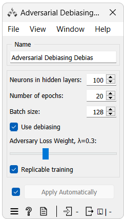
As seen from the image, there are some unique parameters for this widget:

• Neurons in hidden layers: The number of neurons in each of the hidden layers of the neural network.
• Use Debiasing: Whether to use the debiasing or not. The widget will function as a regular neural network model if this option is not selected.
• Adversary loss weight: The weight of the adversary loss in the total loss function. The adversary loss is the loss function of the discriminator. The higher the weight, the more the model will try to reduce the discriminator's ability to predict the protected variable at the expense of the predictor's ability to predict the target variable.

Orange use case

Now that we know how the Adversarial Debiasing widget works and how to use it, let us look at a real-world example for a classification task.

For this example, we will use the Adult dataset, which we have used before. The Adult dataset consists of 48842 instances with 15 attributes describing demographic details from the 1994 census. The primary task is to predict if an individual earns more than $50,000 annually. Unlike previously, we will not use the As Fairness widget to select fairness attributes; instead, we will keep the default ones, "sex" for the protected attribute and "male" for the privileged protected attribute value.

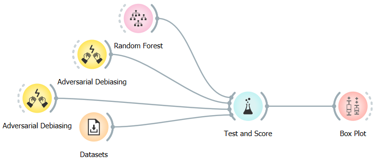
We will train two Adversarial Debiasing models, one with and one without debiasing, and compare them to Random Forests.

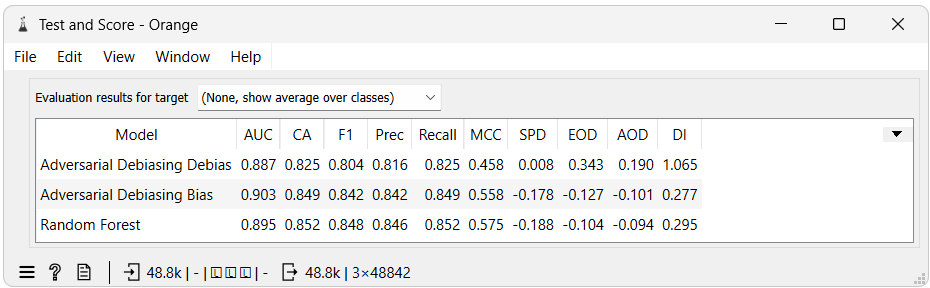
Test and Score shows that debiasing improved fairness metrics, particularly Disparate Impact, and Statistical Parity Difference. Without debiasing, the results are similar to that of the Random Forest model. Disparate Impact moved from 0.277 to 1.065, while Statistical Parity Difference went from -0.178 to 0.008, indicating a near-zero bias between these groups regarding favorable outcomes.

However, this does not mean all forms of bias were addressed. Equal Opportunity Difference and Average Odds Difference metrics worsened from -0.127 to 0.343 and -0.101 to 0.190, respectively. This suggests that even though the algorithm has been optimized for specific fairness criteria, other biases have emerged or become more pronounced.

Why is this happening?

• Trade-offs in fairness: Addressing one type of fairness sometimes comes at the expense of another. When we optimize for Disparate Impact or Statistical Parity Difference, it may affect how often positive outcomes are correctly predicted for both privileged and unprivileged groups (equal opportunity). Moreover, it could alter the balance between true positive rates and false positive rates for these groups (average odds difference).

• Adversarial Debiasing implementation: The current algorithm implementation aims to make predictions independent of protected attributes, focusing on balancing outcomes. This approach inherently focuses on balancing outcomes (reflected in the Disparate Impact and Statistical Parity Difference metrics). However, the nuances of other fairness measures might not be as effectively addressed.

When we use debiasing, there can also be a slight decrease in accuracy. This happens because the model is now not only trying to be accurate but also fair. This balance is a necessary trade-off we accept when we want to remove bias. However, it is worth noting that in this example, the accuracy remains comparable to the scenario without debiasing.

Next, let us look at the Box Plot widget. We will use it to show the Disparate Impact and Statistical Parity Difference, much like our previous blog approach.

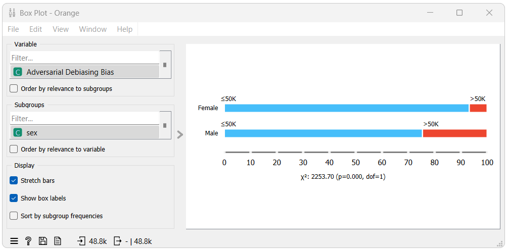
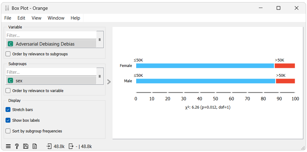
From the first box plot we can see that when using the model without debiasing, males (the privileged group) tends to get classified with ">50K" (the favorable class) more often than females (the unprivileged group) do. This is reflected in the Disparate Impact and Statistical Parity Difference metrics which are 0.277 and -0.178, respectively, both below their optimal value, indicating bias towards the unprivileged group.

In the second box plot, we can see that when using the model with debiasing, males and females get classified with the favorable class at a very similar rate. This is also indicated by the Disparate Impact and Statistical Parity Difference metrics which are 1.065 and 0.008, respectively, both very close to their optimal value, indicating a negligible amount of bias towards the privileged group.