clustering, education, plot
Hierarchical Clustering: A Simple Explanation
AJDA
Dec 02, 2015
One of the key techniques of exploratory data mining is clustering – separating instances into distinct groups based on some measure of similarity. We can estimate the similarity between two data instances through euclidean (pythagorean), manhattan (sum of absolute differences between coordinates) and mahalanobis distance (distance from the mean by standard deviation), or, say, through Pearson correlation or Spearman correlation.
Our main goal when clustering data is to get groups of data instances where:
- each group (Ci) is a a subset of the training data (U): Ci ⊂ U
- an intersection of all the sets is an empty set: Ci ∩ Cj = 0
- a union of all groups equals the train data: Ci ∪ Cj = U
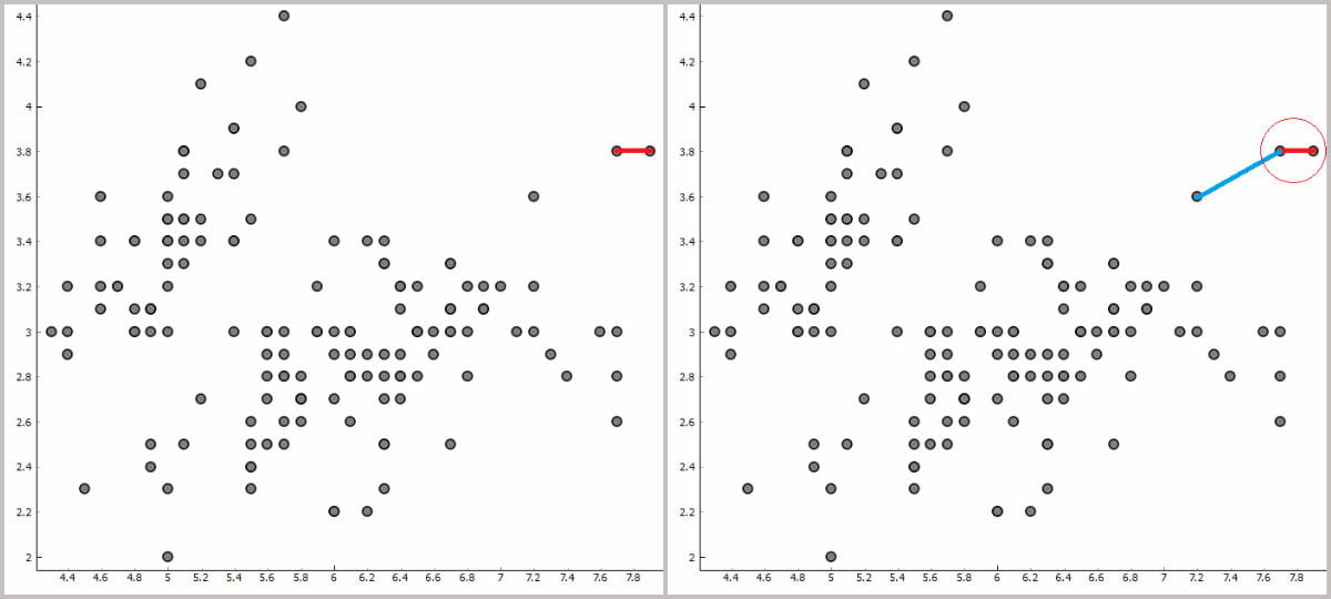
This would be ideal. But we rarely get the data, where separation is so clear. One of the easiest techniques to cluster the data is hierarchical clustering. First, we take an instance from, say, 2D plot. Now we want to find its nearest neighbor. Nearest neighbor of course depends on the measure of distance we choose, but let’s go with euclidean for now as it is the easiest to visualize.
 First steps of hierarchical clustering.
Euclidean distance is calculated as:

Naturally, the shorter the distance the more similar the two instances are. In the beginning, all instances are in their own particular clusters. Then we seek for the closest instances of every instance in the plot. We pin down the closest instance and make a cluster of the original and the closest instance. Now we repeat the process again. What is the closest instances to our new cluster –> add it to the cluster –> find the closest instance. We repeat this procedure until all the instances are grouped in one single cluster.
We can write this down also in a form of a pseudocode:
	every instance is in its own cluster

	repeat until instances are all in one group:

	    find the closest instances to the group (distance has to be minimum)

	    join closest instances with the group

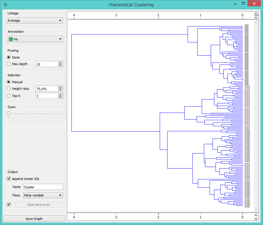
Visualization of this procedure is called a dendrogram, which is what Hierarchical clustering widget displays in Orange.

Single, complete and average linkage.
Another thing to consider is the distance between instances when we have already two or more instances in a cluster. Do we go with the closest instance in a cluster or to the furthest one?
- Picture A shows the distances to the closest instance – single linkage.
- Picture B shows the distance to the furthest instance – complete linkage.
- Picture C shows the average of all distances in a cluster to the instance – average linkage.
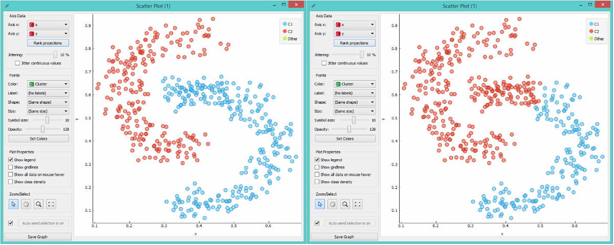
The downside of single linkage is, even by intuition, creating elongated, stretched clusters. Instances at the top part of the red C are in fact quite different from the lower part of the red C. Complete linkage does much better here as it centers clustering nicely. However, the downside of complete linkage is taking outliers too much into consideration. Naturally, each approach has its own pros and cons and it’s good to know how they work in order to use them correctly. One extra hint: single linkage works great for image recognition, exactly because it can follow the curve.
There’s a lot more we could say about hierarchical clustering, but to sum it up, let’s state pros and cons of this method:
- pros: sums up the data, good for small data sets
- cons: computationally demanding, fails on larger sets
