An introduction to the Kaplan-Meier Estimator

The Kaplan-Meier Estimator is a function that relates time to the probability of an event of interest. It is widely used in survival analysis and with the addition of the Survival Analysis package to Orange it is now readily available for accessible visual analytics. However, any kind of efficient data analysis requires a basic understanding of what the implemented model does. This blog post thus aims to:

• explain the most important concepts needed for understanding the Kaplan-Meier Estimator,
• show how to manually calculate and interpret a survival curve to build an intuitive understanding and
• show how this can be implemented in Orange with a few clicks.

Why the need for a special method?

The "survival" in survival analysis gets its name from its use in the analysis of the survival of patients. However, the event of interest can be many things: a disease relapse, the first technical failure of a car, or a user leaving a webpage. There are many real-world problems where we would like to estimate the probability of an event happening in relation to the passing of time. For such estimations, we need a survival dataset, which necessarily includes data instances characterized by the occurrence of an event and the time at which it did.

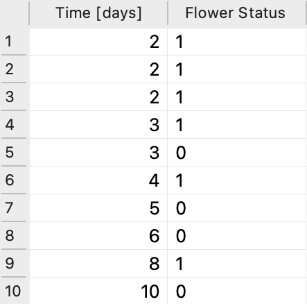
Perhaps the easiest way of getting an understanding of the concepts involved in the estimation of a survival function is with a simple example. Say we get our hands on a tiny dataset from a not-so-grim survival scenario: 10 people received 10 flowers for their birthday and tracked when the flowers wither. The tracking lasted for 10 days. Some flowers wither quicker than others and we are interested in the probability of a flower withering over time. The two main parameters of interest are thus time (in days) and flower withering-status, where "status = 1" means withered and "status = 0" means not-withered. How are we to go about determining the probability of withering over time?

There are two distinct problems when it comes to the analysis of survival:

1. The first one has to do with the fact that "status = 0" does not necessarily mean that the flower has survived. What it does mean is that from that moment on the flower is no longer part of the ongoing study. For instance, a cat might have knocked over the vase and the flower was then discarded along with the broken vase. This does not mean the flower has withered nor that it has survived. We do not want to discard these kinds of data instances, so instead, we label them as censored. This is what "status = 0" really stands for.
2. The second problem has to do with time. First, we do not necessarily have status data available for each day and indeed in our flower dataset we do not - we only have status data for 7 out of 10 days. Furthermore, the effects (for instance, of being without a root) accumulate over time. Even though a flower might have survived for 5 days, its survival probability on day 5 is not 100 %. A decrease in the survival probability also accumulates over time, so it cannot be determined by simply counting the survivors and non-survivors on a particular day.

So which statistical tool should we use?

Although the fact that we have a numeric variable, time, might tempt us to use linear regression this will not be very useful since we just mentioned that the survival probability is non-linear. We might try logistic regression since the probability curve produced by it is not linear and might catch the trend of survival over time better. But logistic regression won't do either. The fifth flower has a status 0 on day 3. As we said before, this does not mean the flower has withered - it only means something happened to it that prevented it from continuing to be part of the study. The probabilities in logistic regression would count this flower as if it survived after the third day, simply because its status is not 1. Thus, logistic regression overestimates survival probability and is therefore also an inappropriate tool to analyze survival data.

This is where the Kaplan-Meier Estimator comes in. It solves both issues, since it models non-linear survival probabilities over time while accounting for subjects of the study who were unable to continue to be part of the study, but did not experience the event of interest. It does so by marking these observances as censored since it is inappropriate to say that the subject (flower) either withered or survived.

Calculating the survival curve manually

Back to our example. Let's imagine 10 people that all have their birthday on the same day. Their mothers, friends, or spouses go and buy them a flower on that day. The probability of a flower withering the day before is probably zero since flower shops don't sell withered flowers. On the day when these freshly cut flowers are sold and given as a gift none of them wither, but the next day three do. From this, we can calculate the probability of withering and the probability of survival for that day. The probability of withering is the number of flowers withered divided by all the flowers that are at risk on that particular day:

Probability of withering: 3/10 = 0.3 = 30%

Probability of surviving: 7/10 = 0.7 = 70%

The probability of surviving is cumulative and so we have to multiply the probability of surviving that day with the previous probability of surviving. Since the probability of withering on the first day was 0 this means the survival probability was 1 and the multiplication does not change anything for the second day.

On the third day, another flower withered and one stopped being part of the experiment for an unknown reason (probably that pesky cat). We have to remove it from the number of flowers at risk of withering for the next day. So while on the third day there are 7 flowers at risk, since 3 withered away the day before, on the fourth day there are only 5 at risk, since the day before one withered away and one got censored for an unknown reason. So the probability of withering on the fourth day is 1/5 and the probability of surviving is 4/5 multiplied by the probability of surviving the previous day, which was 0.6. Let's display all our calculations in a table:

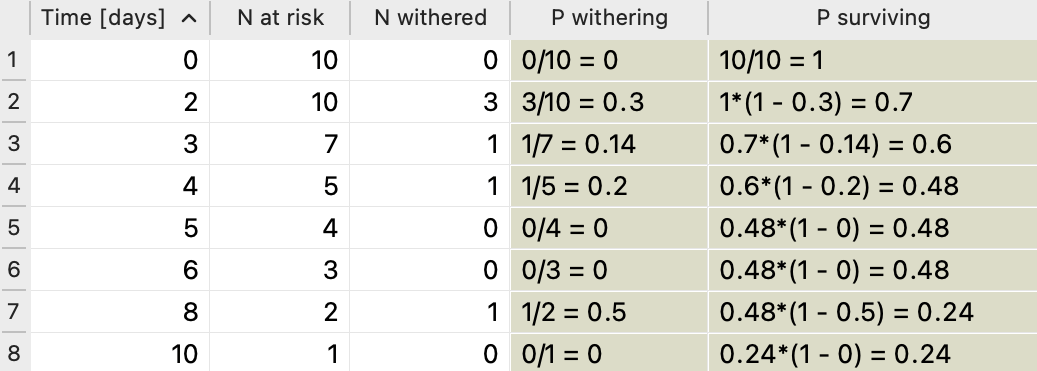
On the 5th and 6th days, none of the remaining flowers withered but two got censored. There is no need to calculate the probability of survival on days where there are only censored data points, but for the sake of clarity, we included the calculations in the table. We can see that the censored data affects the number of flowers at risk but does not change the survival probability. On the eighth day, there are thus only 2 flowers at risk, and one of them withers. Taking into account the survival probability of the previous day this gives us the probability of survival of 0.24.

What would happen if we ignored censored data? We could just exclude them from the analysis but we don't want to do that, because these data points are still informative when it comes to survival. And if we would treat them as surviving we would overestimate the survival probability.

If we plot the survival probability for each day we get the Kaplan-Meier Plot.

Orange use case

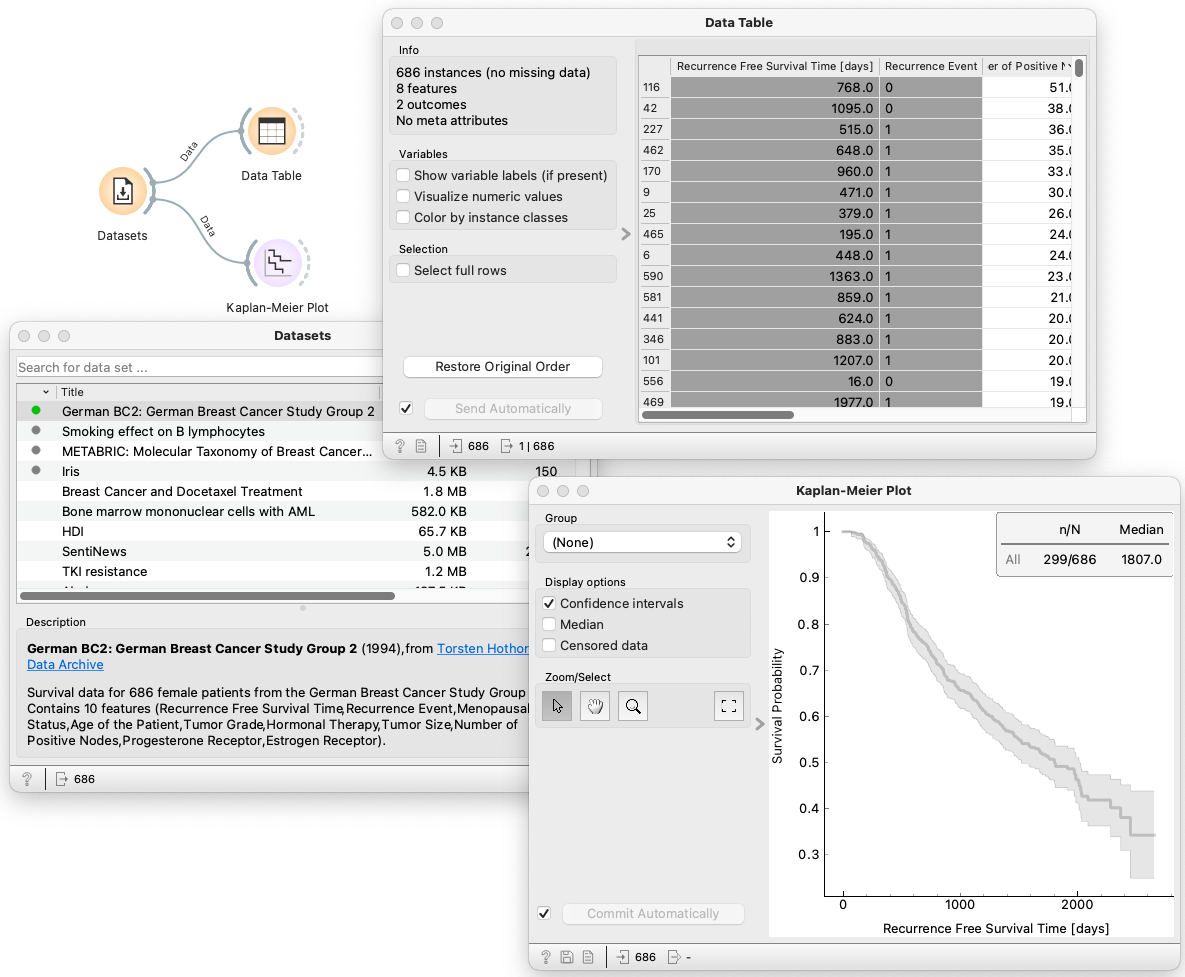
Now that we calculated the Kaplan-Meier estimator on a small dataset manually and got an understanding of what's going on, let's perform this on a larger dataset in Orange. We will use the data from the German Breast Cancer Study Group 2, a survival dataset that is made readily available in Orange. First, we load the data using the Datasets widget and inspect the data in tabular format with the use of Data Table. We see that our data consists of 686 data instances that stand for patients. Each patient is characterized by 8 clinical features and the time at which recurrence of the disease happened or when the patient stopped being part of the experiment due to unknown reasons (censored). We then connect our data with the Kaplan-Meier widget that calculates the survival probability at different time points and plots the survival curve. The widget also allows us to choose one of the three categorical features and compare the survival curves of the different categories.

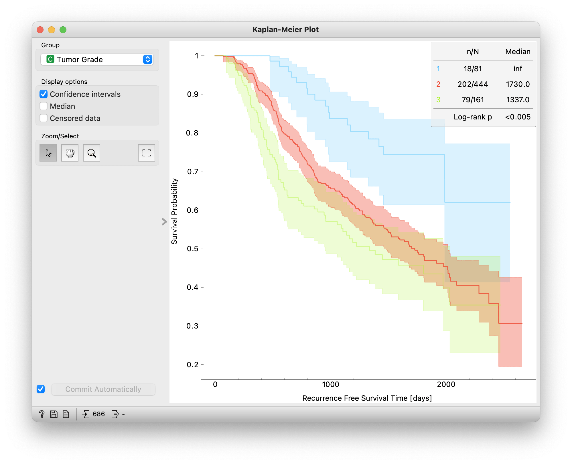
Comparing two or more survival curves can be done by visual inspection or by comparing different statistics. For instance, we can compare the survival curves of patients according to their tumor grade which is a quantitative measure of how abnormal the tumor cells and tissue look under a microscope. For characterizing breast cancer grades doctors most often use the Nottingham grading system which divides the tumor into three grades, where 1 corresponds to low grade, 2 to intermediate grade, and 3 to high grade. The high grade means that the cells and tissue look most abnormal compared to healthy tissue.

We can see this reflected in the survival curves of the three grades: patients with grade 1 tumors have the highest survival probability throughout the study and patients with grade 3 have the lowest. We can also plot the confidence intervals and check if they overlap. The confidence intervals of all three survival curves are separated for the first two years (700 days), meaning that there is probably a significant difference in recurrence of breast cancer between different tumor grades in the first two years.

Finally, we can compare the median survival times of the groups using the Log-Rank test. The null hypothesis is that there is no difference in survival between the two groups and a p-value below 0.05 allows us to reject the null hypothesis and indicates a significant difference. We can see that there indeed is a significant difference in recurrence-free survival time between the three groups. However, the Log Rank test does not tell us among which groups. This too can be done with additional statistics tests but for this blog post, we've covered more than enough.

You now hopefully have a basic understanding of the working of the Kaplan-Meier Estimator and know how to implement it in Orange using just a few clicks.