correlations, NHTS, null hypothesis, p-value, statistics
How to Abuse p-Values in Correlations
Ajda Pretnar
Jan 04, 2019
In a parallel universe, not so far from ours, Orange’s Correlation widget looks like this.
\
\
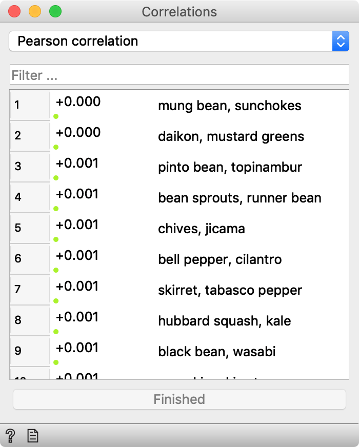
Quite similar to ours, except that this one shows p-values instead of correlation coefficients. Which is actually better, isn’t it? I mean, we have all attended Statistics 101, and we know that you can never trust correlation coefficients without looking at p-values to check that these correlations are real, right? So why on Earth doesn’t Orange show them?
First a side note. It was Christmas not long ago. Let’s call a ceasefire on the frequentist vs. Bayesian war. Let us, for Christ’s sake, pretend, pardon, agree that null-hypothesis testing is not wrong per se.
The mantra of null-hypothesis significance testing goes like this:
- Form hypothesis.
- Collect data.
- Test hypothesis.
In contrast, the parallel-universe Correlation widget is (ab)used like this:
- Collect data.
- Test all possible hypotheses.
- Cherry pick those that are confirmed.
This is like the Texas sharpshooter who fires first and then draws targets around the shots. You should never formulate hypothesis based on some data and then use this same data to prove it. Because it usually (surprise!) works.
\

\
Back to the above snapshot. It shows correlations between 100 vegetables based on 100 different measurements (Ca and Mg content, their consumption in Finland, number of mentions in Star Trek DS9 series, likelihood of finding it on the Mars, and so forth). In other words, it’s all made it up. Just a 100×100 matrix of random numbers with column labels from the simple Wikipedia list of vegetables. Yet the similarity between mung bean and sunchokes surely cannot be dismissed (p < 0.001). Those who like bell pepper should try cilantro, too, because it’s basically one and the same thing (p = 0.001). And I honestly can’t tell black bean from wasabi (p = 0.001).
Here are the p-values for the top 100 most correlated pairs.
import numpy as np import scipy as sp a = np.random.random((100, 100)) sorted(stats.pearsonr(a[i], a[j])[1] for i in range(100) for j in range(i))[:100] [0.0002774329730584203, 0.0004158786523819104, 0.0005008536192579852, 0.0007211022164265075, 0.0008268675086438253, 0.0010265740674904762, (...91 values omitted to reduce the nonsense) 0.01844720610938738, 0.018465602922746942, 0.018662079618069056] First 100 correlations are highly significant.
To learn a lesson we may have failed to grasp at the NHST 101 class, consider that there are 100 * 99 / 2 pairs. What is the significance of the pair at 5-th percentile?
correlations = sorted(stats.pearsonr(a[i], a[j])[1] for i in range(100) for j in range(i)) npairs = 100 * 99 / 2 print(correlations[int(pairs * 0.05)] 0.0496868751692227
Roughly 0.05. This is exactly what should have happened, because:
correlations[int(npairs * 0.10)] 0.10004180592217532 correlations[int(npairs * 0.15)] 0.15236602574520097 correlations[int(npairs * 0.30)] 0.3026816170584785 This proves only that p-values for the Pearson correlation coefficient are well calibrated (and that Mersenne twister that is used to generate random numbers in numpy works well). In theory, the p-value for a certain statistics (like Pearson’s r) is the probability of getting such or even more extreme value if the null-hypothesis (of no correlation, in our case) is actually true. 5 % of random hypotheses should have a p-value below 0.05, 10 % a value below 10, and 23 % a value below 23.
Imagine what they can do with the Correlations widget in the parallel universe! They compute correlations between all pairs, print out the first 5 % of them and start writing a paper without bothering to look at p-values at all. They know they should be statistically significant even if the data is random.
Which is precisely the reason why our widget must not compute p-values: because people would use it for Texas sharpshooting. P-values make sense only in the context of the proper NHST procedure (still pretending for the sake of Christmas ceasefire). They cannot be computed using the data on which they were found.
If so, why do we have the Correlation widget at all if it’s results are unpublishable? We can use it to find highly correlated pairs in a data sample. But we can’t just attach p-values to them and publish them. By finding these pairs (with assistance of Correlation widget) we just formulate hypotheses. This is only step 1 of the enshrined NHST procedure. We can’t skip the other two: the next step is to collect some new data (existing data won’t do!) and then use it to test the hypotheses (step 3).
Following this procedure doesn’t save us from data dredging. There are still plenty of ways to cheat. It is the most tempting to select the first 100 most correlated pairs (or, actually, any 100 pairs), (re)compute correlations on some new data and publish the top 5 % of these pairs. The official solution for this is a patchwork of various corrections for multiple hypotheses testing, but… Well, they don’t work, but we should say no more here. You know, Christmas ceasefire.