addons, business intelligence, gsoc2016, orange3, recommender system
Making recommendations
SALVACARRION
Aug 19, 2016
This is a guest blog from the Google Summer of Code project.
Recommender systems are everywhere, we can find them on YouTube, Amazon, Netflix, iTunes,... This is because they are crucial component in a competitive retail services.
How can I know what you may like if I have almost no information about you? The answer: taking Collaborative filtering (CF) approaches. Basically, this means to combine all the little knowledge we have about users and/or items in order to build a grid of knowledge with which we make recommendation.
To help you with that, Biolab has written Orange3-Recommendation - an add-on for Orange3 to train recommendation models, cross-validate them and make predictions.
Input data
First things first. Orange3-Recommendation can read files in native tab-delimited format, or can load data from any of the major standard spreadsheet file type, like CSV and Excel. Native format starts with a header row with feature (column) names. Second header row gives the attribute type, which can be continuous, discrete, string or time. The third header line contains meta information to identify dependent features (class), irrelevant features (ignore) or meta features (meta).
Here are the first few lines from a data set:
        tid      user        movie       score
        string   discrete    discrete    continuous
        meta     row=1       col=1       class
        1        Breza       HarrySally  2
        2        Dana        Cvetje      5
        3        Cene        Prometheus  5
        4        Ksenija     HarrySally  4
        5        Albert      Matrix      4
        ...
The third row is mandatory in this kind of datasets*, in order to know which attributes correspond to the users (row=1) and which ones to the items (col=1). For the case of big datasets, users and items must be specified as continuous attributes due to efficiency issues. (*Note: If the meta attributes row or col, some simple heuristics will be applied: users=column 0, items=column 1, class=last column)
Here are the first few lines from a data set :
        user            movie         score         tid
        continuous      continuous    continuous    time
        row=1           col=1         class         meta
        196             242           3             881250949
        186             302           3             891717742
        22              377           1             878887116
        244             51            2             880606923
        166             346           1             886397596
        298             474           4             884182806
        ...
Training a model
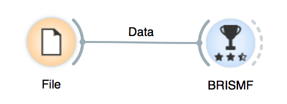
This step is pretty simple. To train a model we have to load the data as is described above and connect it to the learner. (Don't forget to click apply)
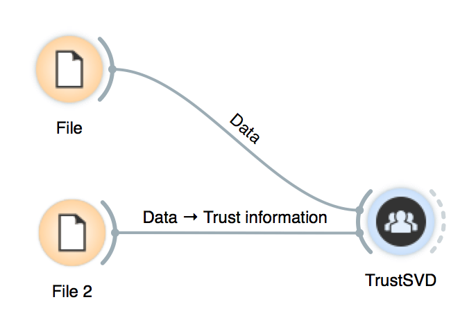
If the model uses side information, we only need to add an extra file.
In addition, we can set the parameters of our model by double-clicking it:
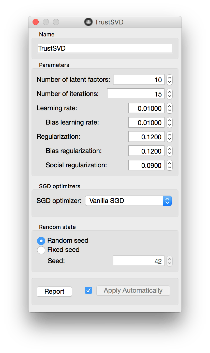
By using a fixed seed, we make random numbers predictable. Therefore, this feature is useful if we want to compare results in a deterministic way.
Cross-validation
This is as simple as it seems. The only thing to point out is that side information must be connected to the model.
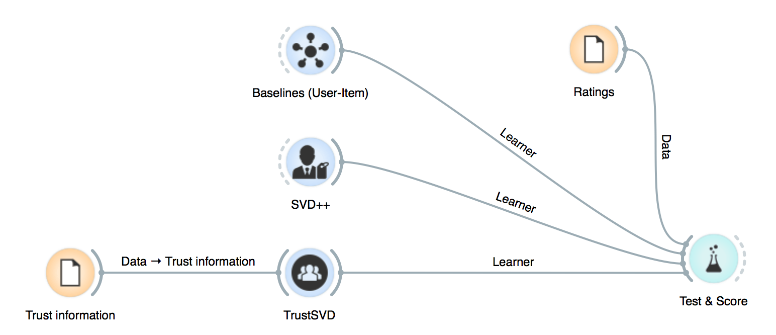
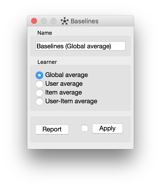
Still, cross-validation is a robust way to see how our model is performing. I consider that it's a good idea to check how our model performs with respect to the baseline. This presents a negligible overload* in our pipeline and makes our analysis more solid. (*For 1,000,000 ratings, it can take 0.027s).
We can add a baseline leaner to Test&Score and select the model we want to apply.
Making recommendations
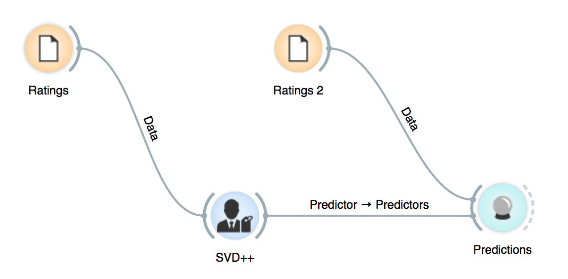
The prediction flow is exactly the same as in Orange3.
Analyzing low-rank matrices
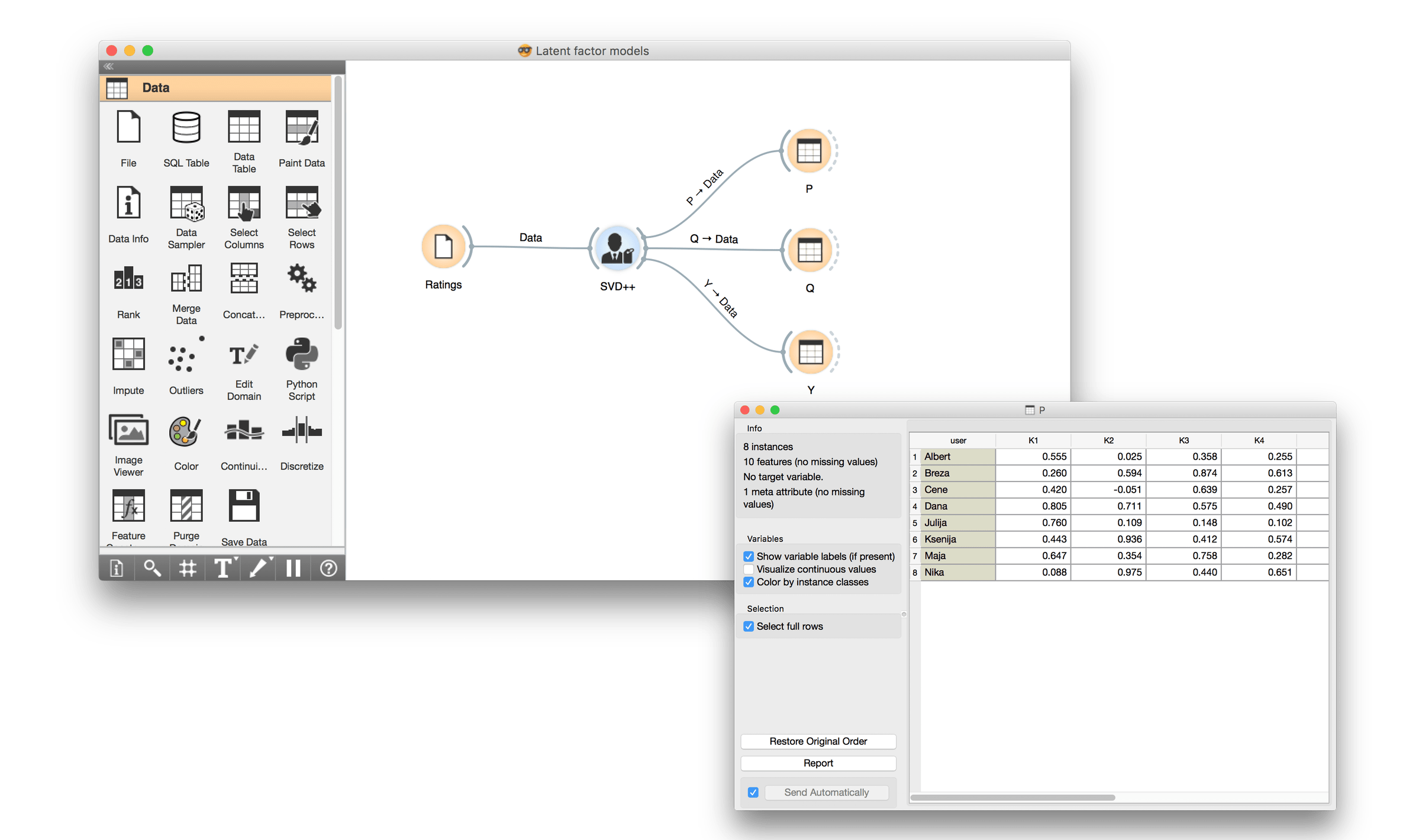
Once we've output the low-rank matrices, we can play around the vectors in those matrices to discover hidden relations or understand the known ones. For instance, here we plot vector 1 and 2 from the item-feature matrix by simply connecting Data Table with selected instances to the widget Scatter Plot.
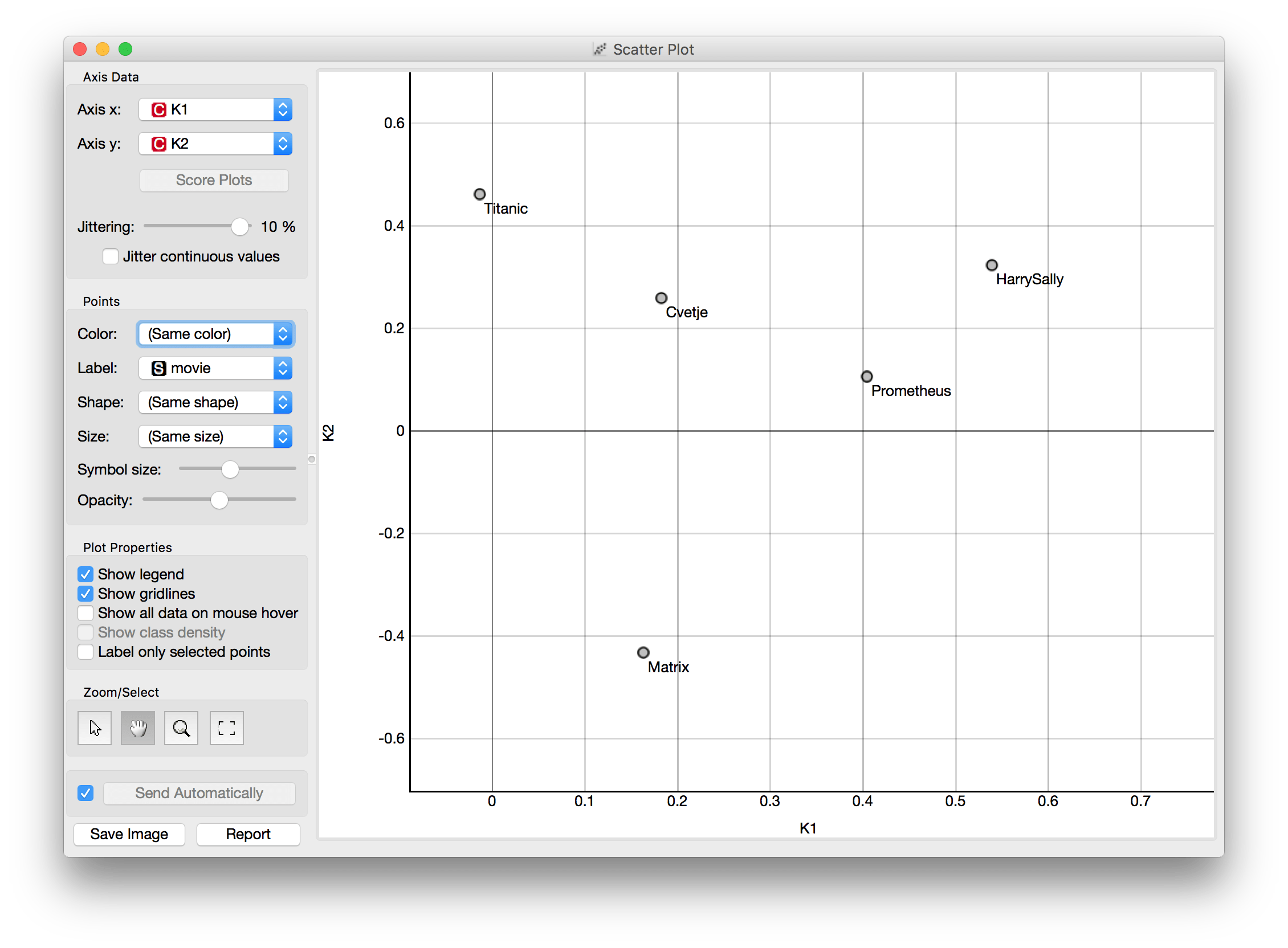
Using similar approaches we can discover pretty interesting things like similarity between movies or users, how movie genres relate with each other, changes in users' behavior, when the popularity of a movie has been raised due to a commercial campaign,... and many others.
Finally, a simple pipeline to do all of the above can be something like this:
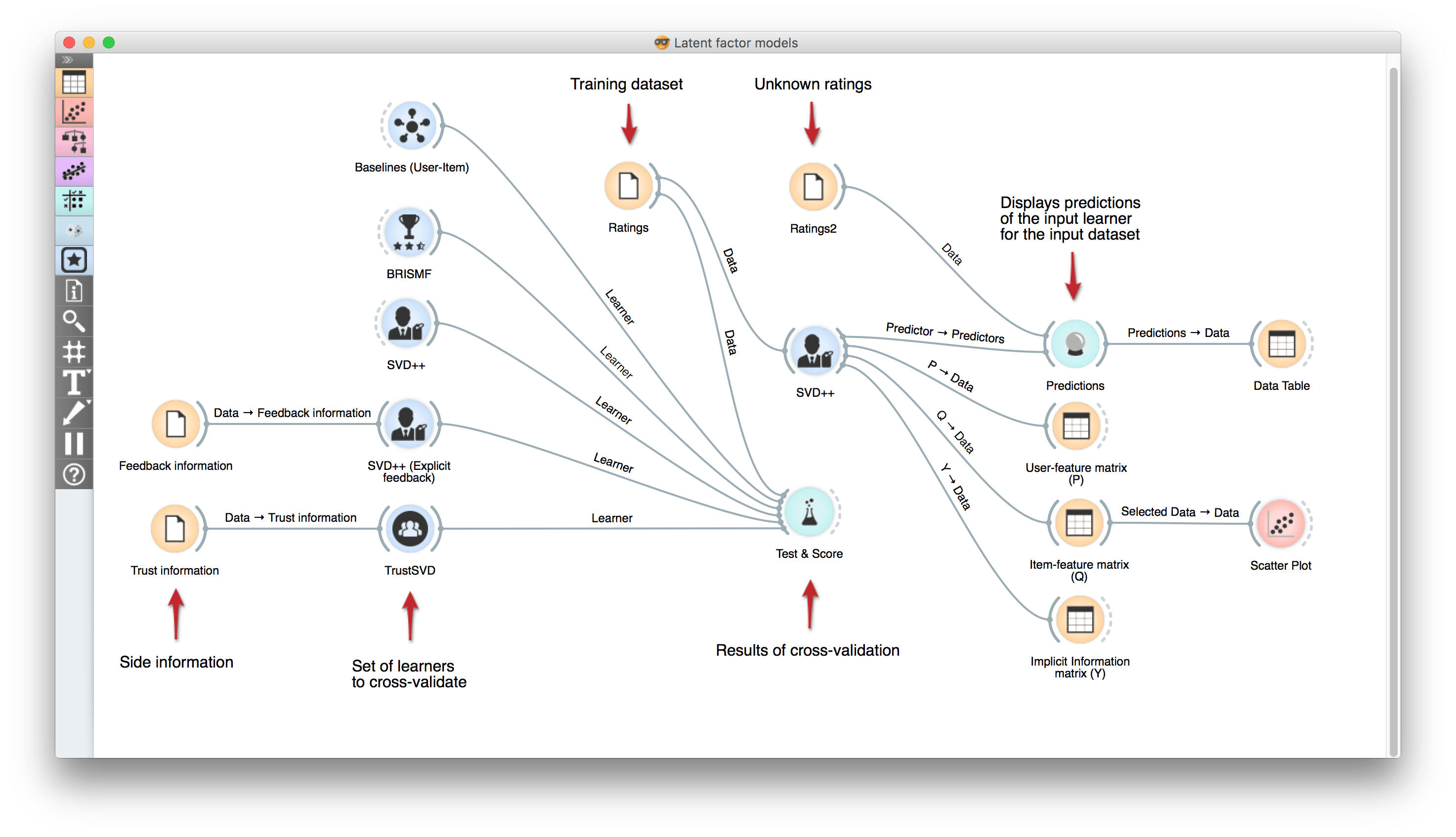
On the left side we connected several models to Test&Score in order to cross-validate them. Later, we trained a SVD++ model, made some predictions, got the low-rank matrices learnt by the model and plotted some vectors of the Item-feature matrix.
Analysis (Advanced users)
Here we've made a workflow (which can be downloaded here) to perform a really basic analysis on the results obtained through factoring the user and item feature matrices with BRISMF over the movielens100k dataset. (Note: Once downloaded, set the prepared datasets in the folder 'orange'. Probably you're gonna get a couple errors. Don't worry, it's normal. To solve it, apply the scripts sequentially but don't forget previously to select all the rows in the related Table.)
Instead of explaining how this pipeline works, the best thing you can do is to download it and play with it.
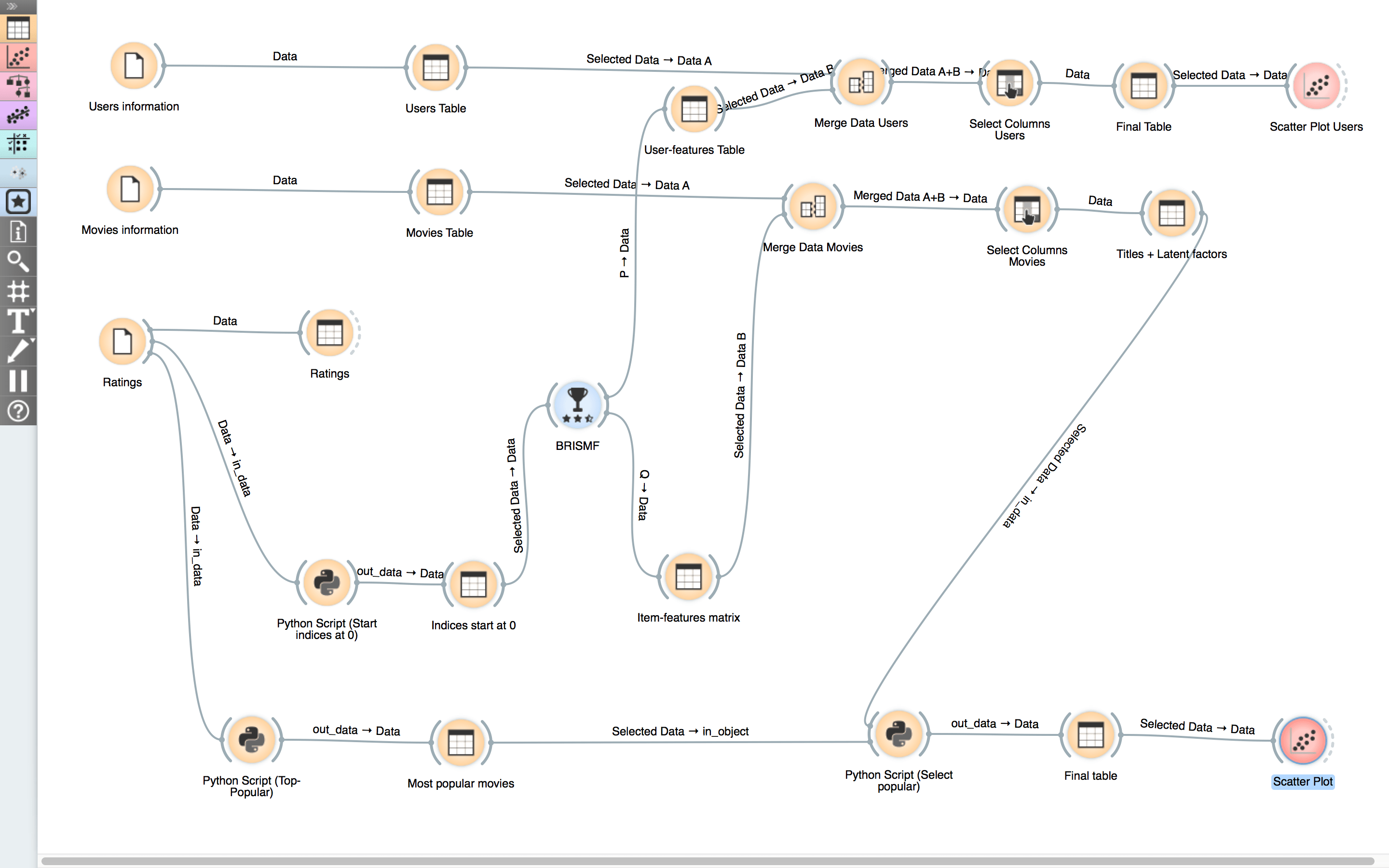
One of the analysis you can do, is to plot the most popular movies across two first vectors of the matrix descomposition. Later, you can try to find clusters, tweak it a bit and find crossed relations (e.g. male/female Vs._ action/drama)._
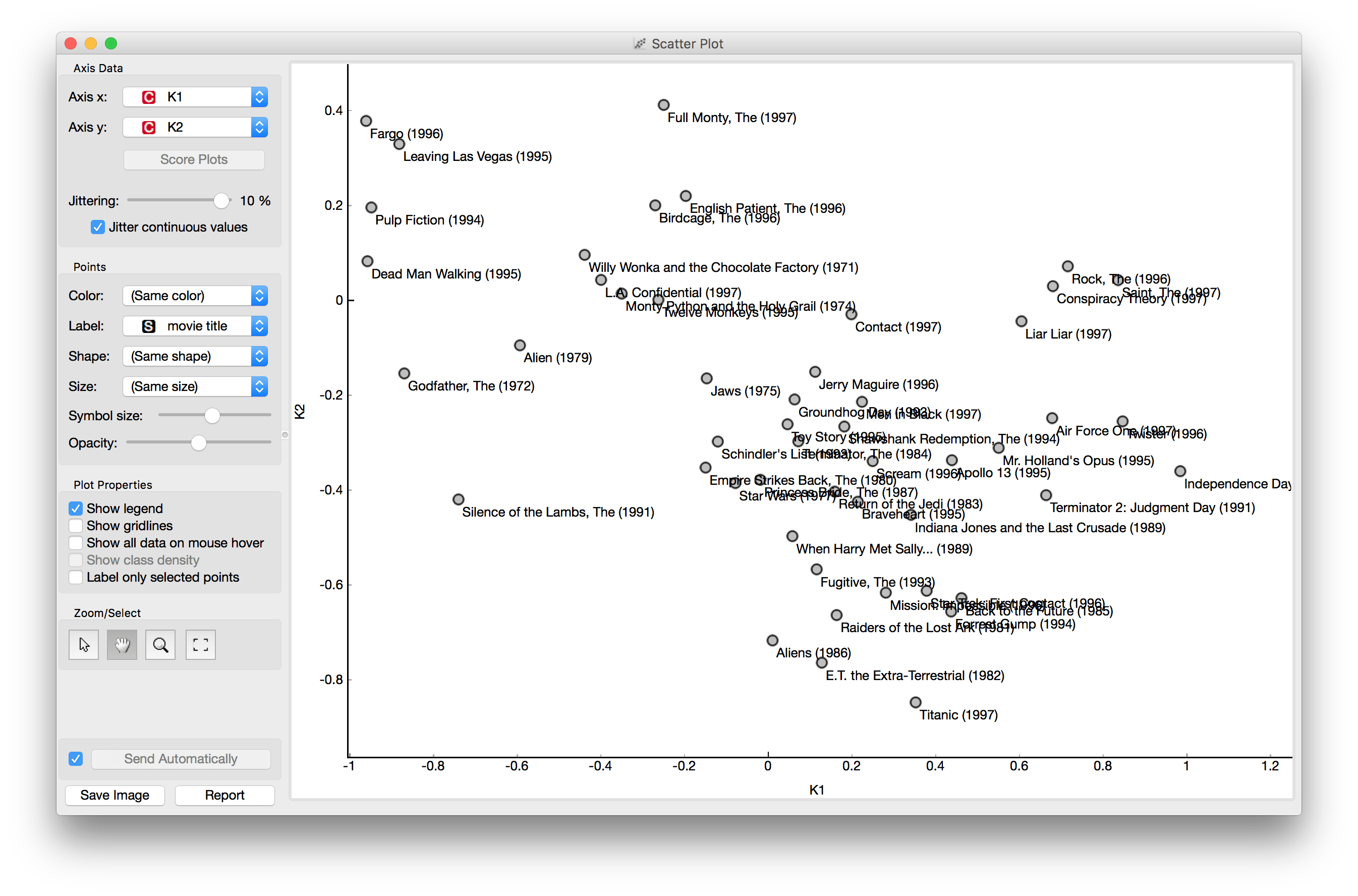
Now let's focus on the scripting part.
Rating models
In this tutorial we are going to train a BRISMF model.
- First we import Orange and the learner that we want to use:
        import Orange
        from orangecontrib.recommendation import BRISMFLearner
- After that, we have to load a dataset:
data = Orange.data.Table('movielens100k.tab')
- Then we set the learner parameters, and finally we train it passing the dataset as an argument (the returned value will be our model trained):
        learner = BRISMFLearner(num_factors=15, num_iter=25, learning_rate=0.07, lmbda=0.1)
        recommender = learner(data)
- Finally, we can make predictions (in this case, for the first three pairs in the dataset):
        prediction = recommender(data[:3])
        print(prediction)
        >>> [ 3.79505151 3.75096513 1.293013 ]
Ranking models
At this point we can try something new, let's make recommendations for a dataset in which only binary relevance is available. For this case, CLiMF is model that will suit our needs.
    import Orange
    import numpy as np
    from orangecontrib.recommendation import CLiMFLearner

    # Load data
    data = Orange.data.Table('epinions_train.tab')

    # Train recommender
    learner = CLiMFLearner(num_factors=10, num_iter=10, learning_rate=0.0001, lmbda=0.001)
    recommender = learner(data)

    # Make recommendations
    recommender(X=5)
    >>> [ 494,   803,   180, ..., 25520, 25507, 30815]
Later, we can score the model. In this case we're using the MeanReciprocalRank:
    import Orange

    # Load test
    dataset testdata = Orange.data.Table('epinions_test.tab')

    # Sample users
    num_users = len(recommender.U)
    num_samples = min(num_users, 1000) # max. number to sample
    users_sampled = np.random.choice(np.arange(num_users), num_samples)

    # Compute Mean Reciprocal Rank (MRR)
    mrr, _ = recommender.compute_mrr(data=testdata, users=users_sampled)
    print('MRR: %.4f' % mrr)
    >>> MRR: 0.3975
SGD optimizers
This add-on includes several configurations that can be used to modify the updates on the low rank matrices during the stochastic gradient descent optimization.
- SGD: Classical SGD update.
- Momentum: SGD with inertia.
- Nesterov momentum: A Momentum that "looks ahead".
- AdaGrad: Optimizer that adapts its learning rating during the process.
- RMSProp: "Leaky" AdaGrad.
- AdaDelta: Extension of Adagrad that seeks to reduce its aggressive.
- Adam: Similar to AdaGrad and RMSProp but with an exponentially decaying average of past gradients.
- Adamax: Similar to Adam, but taking the maximum between the gradient and the velocity.
Do you want to learn more about this? Check our documentation!